Introduction

In this tab, we tried to build Rumor Detection A classification method called SVM(Supported Vector Machine) will be used. The data set included is “cleaned_supervised_data.csv”

Theroy

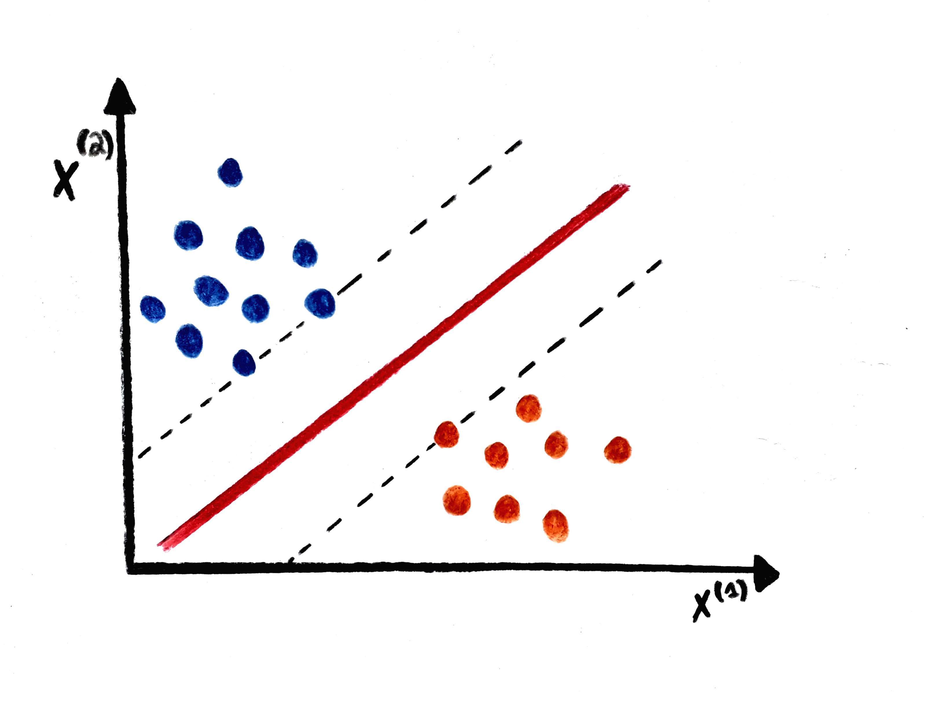
SVM “draw a bound” at the middle of the distance between the closest two samples.

(Example how svm functions)

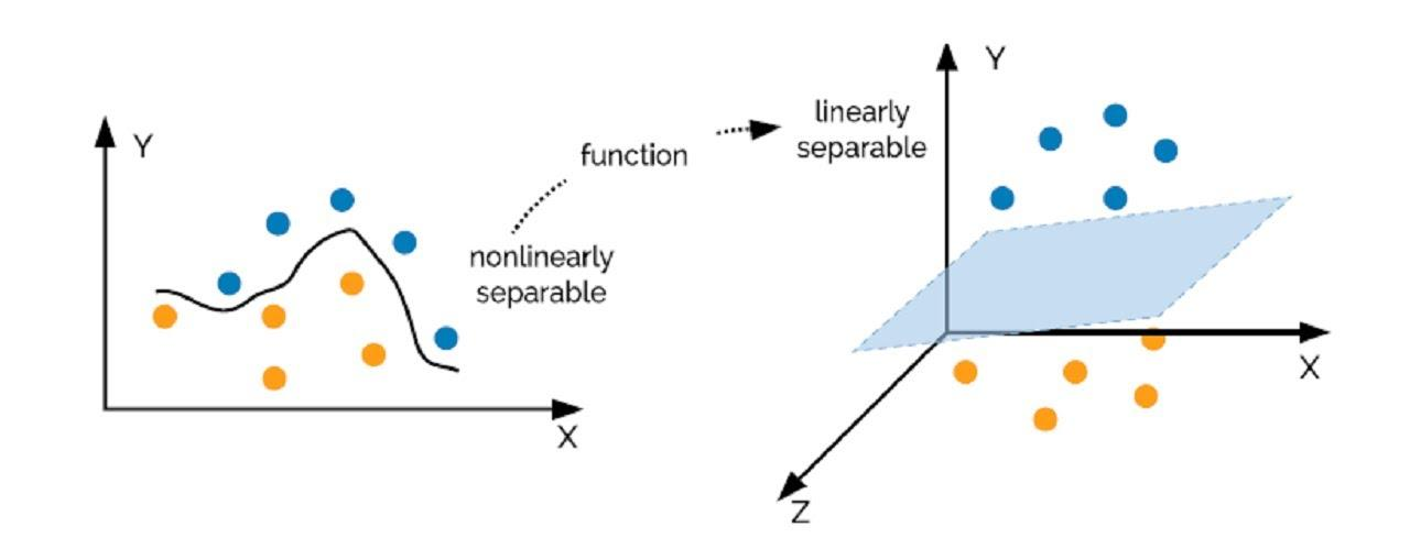
Beside, by appling “kernel trick”, SVM can also draw non-linear lines to seperate points.

(Example how kernel svm functions)

Advantages of this method is: SVM performs reasonably well when the difference between classes is huge.

Method

This part will show the workflow of training the optimal models with SVM.

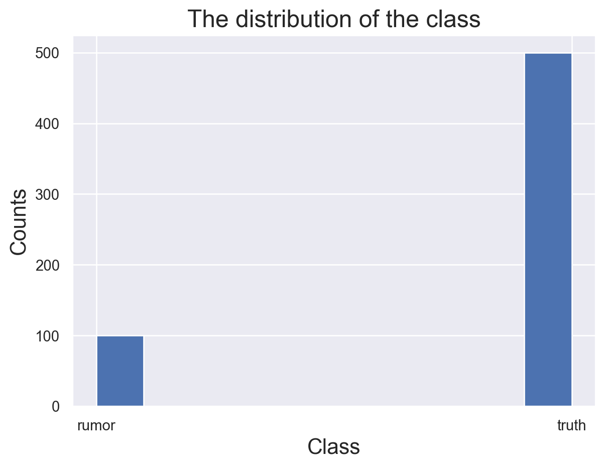
Class Distribution

Code

# import libraries
import numpy as np
import pandas as pd
import matplotlib.pyplot as plt
import seaborn as sns
from sklearn.svm import SVC
from sklearn.model_selection import GridSearchCV
from sklearn.model_selection import train_test_split
from sklearn.feature_extraction.text import CountVectorizer
from sklearn.metrics import accuracy_score
from sklearn.metrics import precision_recall_fscore_support
from sklearn.metrics import precision_score
from sklearn.metrics import recall_score
from sklearn.metrics import confusion_matrix
#set the seed 
np.random.seed(1)
#load the data 
df=pd.read_csv("../../data/01-modified-data/supervised_data.csv")
y=df["label"]
#plot the distribution of two classes
sns.set_theme()
plt.hist(y)
plt.title("The distribution of the class",fontsize=18)
plt.xlabel("Class",fontsize=16)
plt.ylabel("Counts",fontsize=16)
df.head()

	text	location	friends_count	followers_count	screen_name	retweet_count	favorite_count	label	description
0	is that you tome hanks?...how about we keep am...	NaN	12269	39845	helen henning	763	4208	rumor	MAKE AMERICA FLORIDA...let's have some fun...s...
1	After the dreadful hurricane in Florida @VP K...	London	34500	36867	David Atherton	198	297	rumor	Libertarian, free markets, free speech. "Selfi...
2	Heartbreaking! Iranian father who promised to ...	Iraq	1619	9009	Shukri Hamk	9589	30927	rumor	-Survivor of #YazidiGenocide. -human rights ac...
3	my dad just sent me this video from Naples Flo...	NaN	72	32	the worlds foremost authority	933	3681	rumor	it’s just a cope fest
4	Omg so all funerals due on the 19 th have been...	NaN	4995	4080	Carolyn Brown	3381	26141	rumor	Feminist, Cymraes and European! 🏴󠁧󠁢󠁷󠁬󠁳󠁿🇪🇺🏴󠁧󠁢󠁳󠁣...

This is an imbalanced data, the number of truth is bigger than the number of rumor. This is induced by two different ways of collecting data. Rumor samples are rather hard to get. In this model, we will try to use sample a equal number of truth from the rows where label is “truth”.

Baseline Model for Comparsion

Code

# transform the label 
y=y.str.replace("rumor","1")
y=y.str.replace("truth","0")
y=y.astype("int")
#set a baseline model which random predict label
def random_classifier(y_data):
    ypred=[]
    max_label=np.max(y_data); #print(max_label)
    for i in range(0,len(y_data)):
        ypred.append(int(np.floor((max_label+1)*np.random.uniform(0,1))))
    print("-----RANDOM CLASSIFIER-----")
    print("accuracy",accuracy_score(y_data, ypred))
    print("percision, recall, fscore,",precision_recall_fscore_support(y_data,ypred))

random_classifier(y)

-----RANDOM CLASSIFIER-----
accuracy 0.4766666666666667
percision, recall, fscore, (array([0.82291667, 0.15705128]), array([0.474, 0.49 ]), array([0.60152284, 0.23786408]), array([500, 100], dtype=int64))

What a baseline model here did is guess the class. And we can see that every metric is around 50%. So if a model perform than this baseline, than we can say it do make some sense.

Feature Selection

Code

#sample a subset of negative samples
a=df[df["label"]=="truth"].sample(100)
b=df[df['label']=="rumor"]
df=pd.concat([a,b])
df.reset_index(drop=True, inplace=True)
y=df['label']
X=df["text"]
y=y.str.replace("rumor","1")
y=y.str.replace("truth","0")
y=y.astype("int")
#transform texts with countvectorizer
vectorizer = CountVectorizer()
matrix = vectorizer.fit_transform(X)
X = pd.DataFrame(matrix.toarray(),columns=vectorizer.get_feature_names_out())
#split the data
x_train,x_test,y_train,y_test=train_test_split(X,y,test_size=0.2)

This model try to use texts to classify, so our features are texts transformed by “CountVectorizer”

Model tuning

Code

#find the best hyperparametres with GridSearchCV library
parameter=[
    {"C":[1,10,100,1000],"kernel":["linear"]},
    {"C":[1,10,100,1000],"kernel":["rbf"],"gamma":[0.1,.2,.3,.4,.5,.6,.7,.8,.9]}
]
grid_search = GridSearchCV(SVC(), param_grid=parameter, scoring="accuracy",cv=10)
grid_search=grid_search.fit(X, y)
print("The best hyperparametres are:",grid_search.best_params_)
grid_search

The best hyperparametres are: {'C': 1, 'kernel': 'linear'}

GridSearchCV(cv=10, estimator=SVC(),
             param_grid=[{'C': [1, 10, 100, 1000], 'kernel': ['linear']},
                         {'C': [1, 10, 100, 1000],
                          'gamma': [0.1, 0.2, 0.3, 0.4, 0.5, 0.6, 0.7, 0.8,
                                    0.9],
                          'kernel': ['rbf']}],
             scoring='accuracy')

In a Jupyter environment, please rerun this cell to show the HTML representation or trust the notebook.
On GitHub, the HTML representation is unable to render, please try loading this page with nbviewer.org.

In this part, we use “GridSearchCV” function to help us find the beset parametres so that we don’t need to write codes and make some loops manually. The result shows that we should use linear kernel and should set C as 1.

Final Results

Code

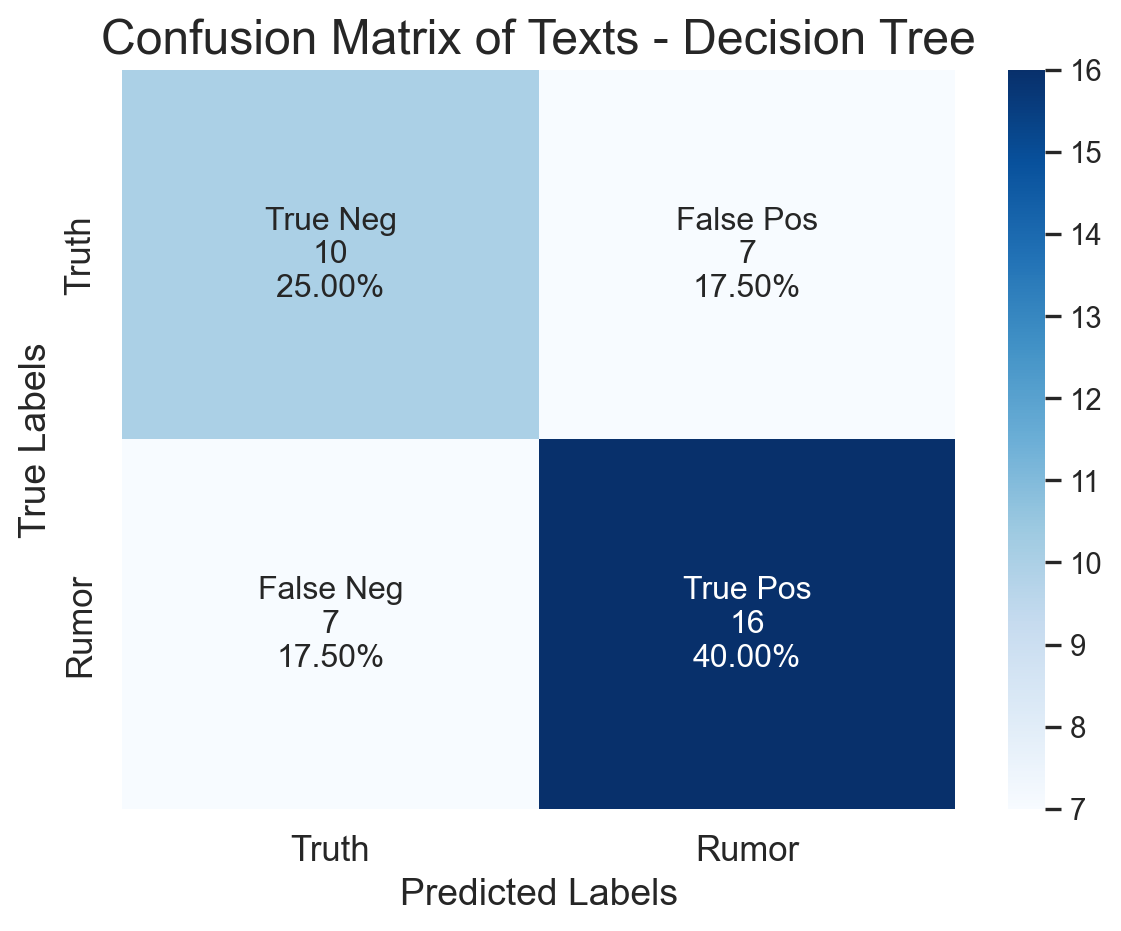
#write a function to report and plot the metrics and confusion matrix.
def confusion_plot(y_data,y_pred):
    print(
        "ACCURACY: "+str(accuracy_score(y_data,y_pred))+"\n"+
        "NEGATIVE RECALL (Y=0): "+str(recall_score(y_data,y_pred,pos_label=0))+"\n"+
        "NEGATIVE PRECISION (Y=0): "+str(precision_score(y_data,y_pred,pos_label=0))+"\n"+
        "POSITIVE RECALL (Y=1): "+str(recall_score(y_data,y_pred,pos_label=1))+"\n"+
        "POSITIVE PRECISION (Y=1): "+str(precision_score(y_data,y_pred,pos_label=1))+"\n"
    )
    cf=confusion_matrix(y_data, y_pred)
    # customize the anno
    group_names = ["True Neg","False Pos","False Neg","True Pos"]
    group_counts = ["{0:0.0f}".format(value) for value in cf.flatten()]
    group_percentages = ["{0:.2%}".format(value) for value in cf.flatten()/np.sum(cf)]
    labels = [f"{v1}\n{v2}\n{v3}" for v1, v2, v3 in zip(group_names,group_counts,group_percentages)]
    labels = np.asarray(labels).reshape(2,2)
    #plot the heatmap
    fig=sns.heatmap(cf, annot=labels, fmt="", cmap='Blues')
    plt.title("Confusion Matrix of Texts - Decision Tree",fontsize=18)
    fig.set_xticklabels(["Truth","Rumor"],fontsize=13)
    fig.set_yticklabels(["Truth","Rumor"],fontsize=13)
    fig.set_xlabel("Predicted Labels",fontsize=14)
    fig.set_ylabel("True Labels",fontsize=14)
    plt.show()
#fit the model with the best hyperparametres
clf=SVC(C=1,kernel="linear")
clf.fit(x_train,y_train)
yp_test=clf.predict(x_test)
confusion_plot(y_test,yp_test)

ACCURACY: 0.65
NEGATIVE RECALL (Y=0): 0.5882352941176471
NEGATIVE PRECISION (Y=0): 0.5882352941176471
POSITIVE RECALL (Y=1): 0.6956521739130435
POSITIVE PRECISION (Y=1): 0.6956521739130435

It seems that even we have used the best hyperparametre, however, the effect of svm is still bad. We can not confidently make judgement basde on this model, since it can hardly distinguish positive samples.

Conclusion

It turns out SVM is not suitable for our topic,performs much worse than naive bayes when facing the same task. The reason may be that we haven’t collected enought data.

Comparing to the naive bayes model, it seems naive bayes still outperform SVM on this task even though its a simple model.