decision

Introduction

In this tab, a classification method called Decision Tree is used to build Susceptible User Detection. We will use “cleaned_followers.csv”.

Theory

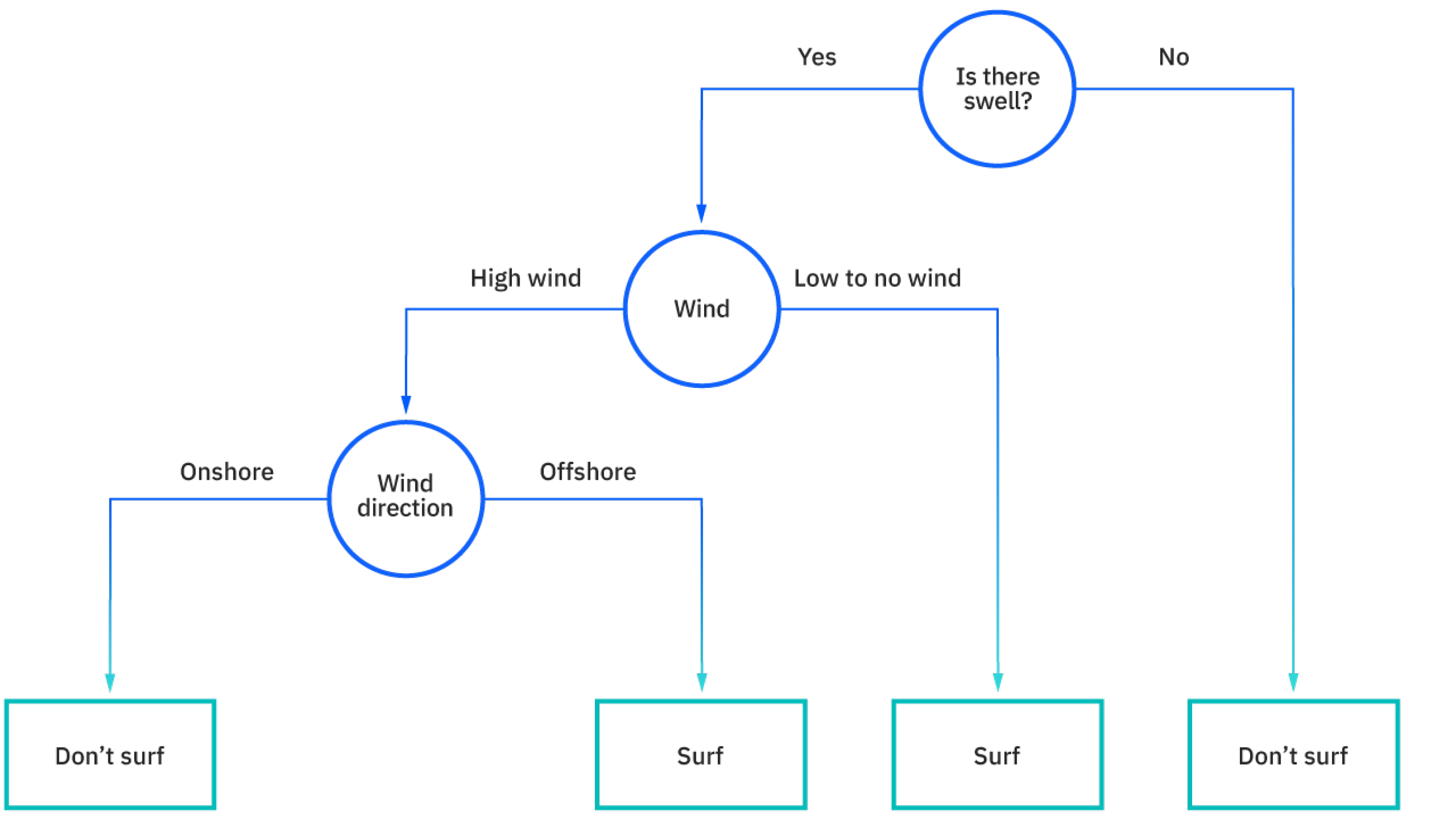
Decision Tree continuouslly asks “whether or not questions” to the input so that it can gradually divides it into different parts.

But how to decide what to ask? The trick here is to use mathematical formulas to quantify one of the following metrics to find the question.

The extent to which we gain new information from new answers (by calculating entropy)

The probability which we incorrectly classify the sample (by calculating gini index)

By using this method, we can easily find how important an attribute is, and understand what makes our research target so different.

Method

This part will show the workflow of training the optimal models with SVM.

Class Distribution

Code

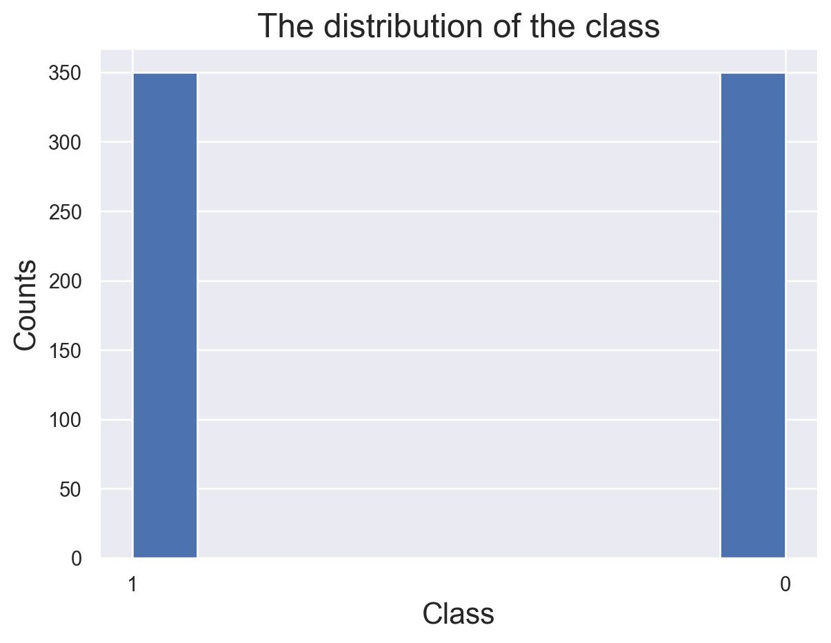
# import libraries
import numpy as np
import pandas as pd
import matplotlib.pyplot as plt
import seaborn as sns
from sklearn import tree
from sklearn.model_selection import train_test_split
from sklearn.metrics import accuracy_score
from sklearn.metrics import precision_recall_fscore_support
from sklearn.metrics import precision_score
from sklearn.metrics import recall_score
from sklearn.metrics import confusion_matrix
#load the data
df=pd.read_csv("../../data/01-modified-data/cleaned_followers.csv")
sns.set_theme()
#plot the distribution
plt.hist(df.label.astype("string"))
plt.title("The distribution of the class",fontsize=18)
plt.xlabel("Class",fontsize=16)
plt.ylabel("Counts",fontsize=16)
#show the data
df.head()

	user_id	screen_name	followers_count	friends_count	listed_count	favourites_count	tweet_num	label
0	2198516225	_Banzi_	27	199	0	601	122	1
1	1504258025804210176	DelorbeTori	81	2771	0	0	6	1
2	1581474148571877377	omkarVyawahare2	0	56	0	24	0	1
3	2967681610	L1BERTE_S	50	68	1	8735	2238	1
4	1400890434	mistamomo_	356	1104	19	18347	20160	1

The count of two classes are the same, 350 for each. This is dsigned when gathering the data(“details of followers”). With this kind of data, we can avoid problems brought from imbalanced data sets.

Baseline Model for Comparsion

Code

#define a baseline model which random assign labels
def random_classifier(y_data):
    ypred=[]
    max_label=np.max(y_data); #print(max_label)
    for i in range(0,len(y_data)):
        ypred.append(int(np.floor((max_label+1)*np.random.uniform(0,1))))
    print("-----RANDOM CLASSIFIER-----")
    print("accuracy",accuracy_score(y_data, ypred))
    print("percision, recall, fscore,",precision_recall_fscore_support(y_data,ypred))

random_classifier(df.label)

-----RANDOM CLASSIFIER-----
accuracy 0.5
percision, recall, fscore, (array([0.5, 0.5]), array([0.50857143, 0.49142857]), array([0.50424929, 0.49567723]), array([350, 350], dtype=int64))

What a baseline model here did is guess the class. And we can see that every metric is around 50%. So if a model perform than this baseline, than we can say it do make some sense.

Data Selection

Code

# id reflect the time account exits,we normalized it 
df["user_id"]=(df.user_id-df.user_id.mean())/df.user_id.std() 
#drop the feature we won't consider about
df.drop(columns=["screen_name"],axis=1,inplace=True)
#
X=df.drop(columns=["label"],axis=1)
y=df["label"]
x_train,x_test,y_train,y_test=train_test_split(X,y,test_size=0.2,random_state=42)

Feature	Meaning
user_id	the id of users
followers_count	the number of followers this account currently has
friends_count	the number of users this account is following
listed_count	the number of public lists that this user is a member of
favourites_count	the number of Tweets this user has liked in the account’s lifetime
tweet_num	the number of Tweets (including retweets) issued by the user
protected	whether user has chosen to protect their Tweets
verified	whether user has a verified account

(The names and meanings of features)

8 features was selected to train the model. These features are all attributes that are allowed to get and reflect the character of accounts. With these attributes, we have the biggest possibility to find the differences. Note that “user_id” is also selected because it reflect how long an account was created. The bigger an user id is, the newer the account is.

Model tuning

Code

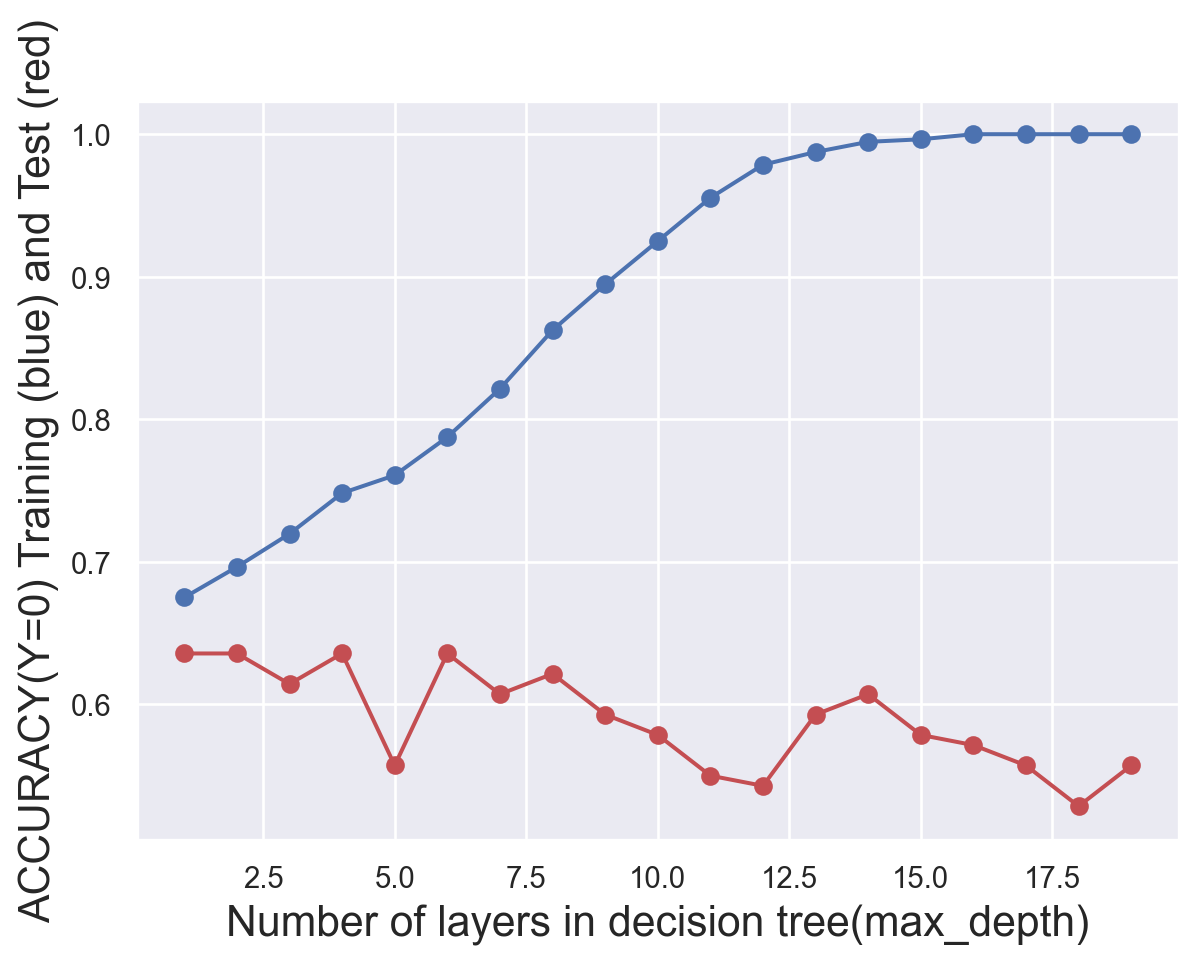
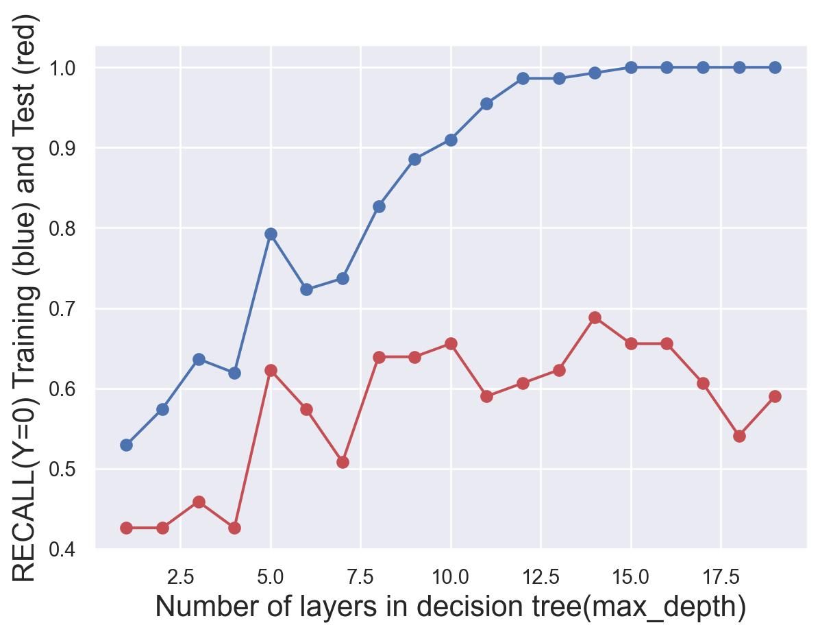
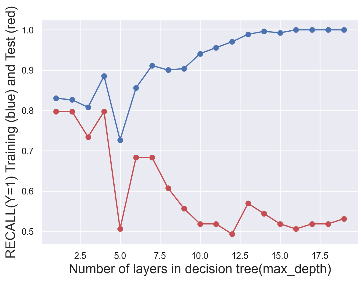
# try different numbers of layers to find the best one
test_results=[]
train_results=[]

for num_layer in range(1,20):
    model = tree.DecisionTreeClassifier(max_depth=num_layer)
    model = model.fit(x_train,y_train)

    yp_train=model.predict(x_train)
    yp_test=model.predict(x_test)

    # print(y_pred.shape)
    test_results.append([num_layer,accuracy_score(y_test, yp_test),recall_score(y_test, yp_test,pos_label=0),recall_score(y_test, yp_test,pos_label=1)])
    train_results.append([num_layer,accuracy_score(y_train, yp_train),recall_score(y_train, yp_train,pos_label=0),recall_score(y_train, yp_train,pos_label=1)])
test_results=np.array(test_results)
train_results=np.array(train_results)
#generate plots of the performance of different layers 
def metric_plot(ylabel,layer,yptrain,yptest):
    fig=plt.figure()
    plt.plot(layer,yptrain,'o-',color="b")
    plt.plot(layer,yptest,'o-',color="r")
    plt.ylabel(ylabel+" Training (blue) and Test (red)",fontsize=16)
    plt.xlabel("Number of layers in decision tree(max_depth)",fontsize=16)
metric_plot("ACCURACY(Y=0)",test_results[:,0],train_results[:,1],test_results[:,1])
metric_plot("RECALL(Y=0)",test_results[:,0],train_results[:,2],test_results[:,2])
metric_plot("RECALL(Y=1)",test_results[:,0],train_results[:,3],test_results[:,3])

To find the most suitable number of layers, several plots was produced. We finally find that we should set max_depth as 4.

Final Results

Code

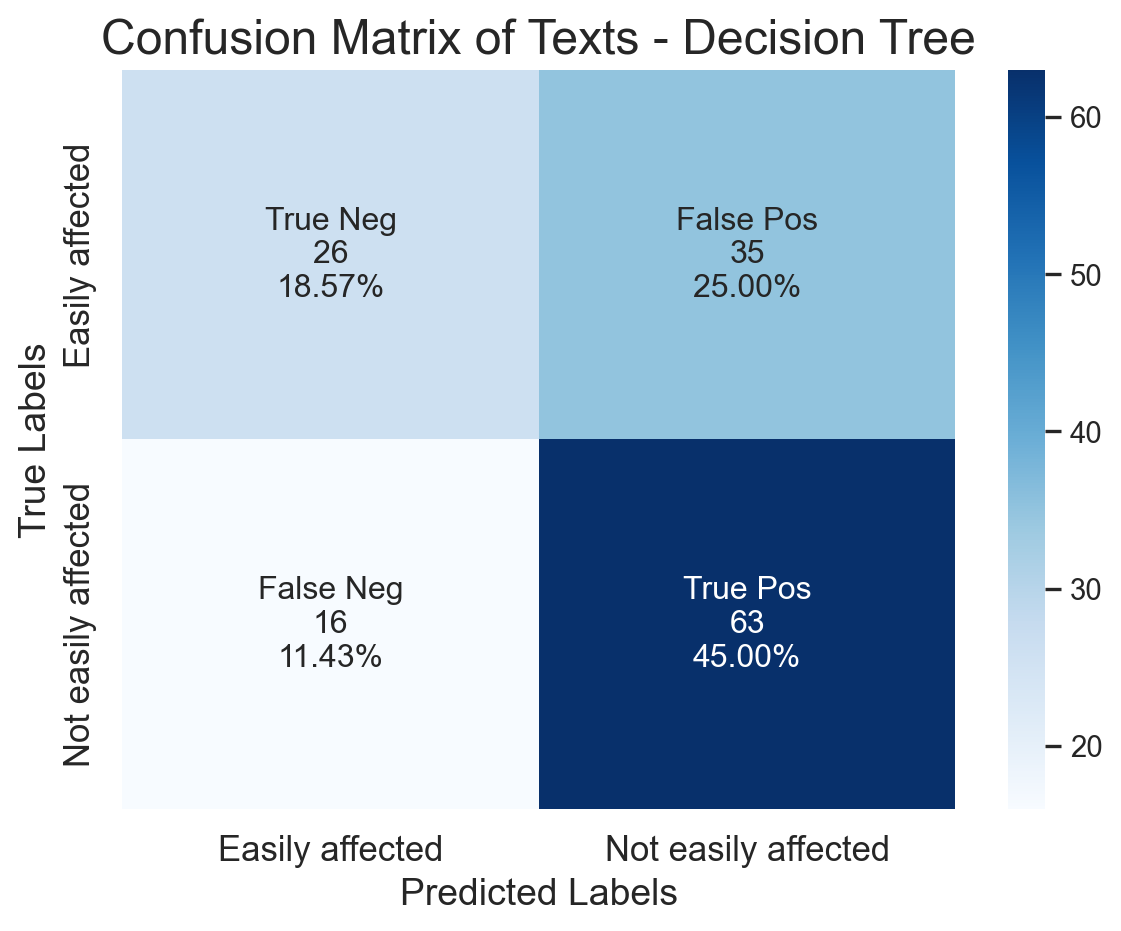
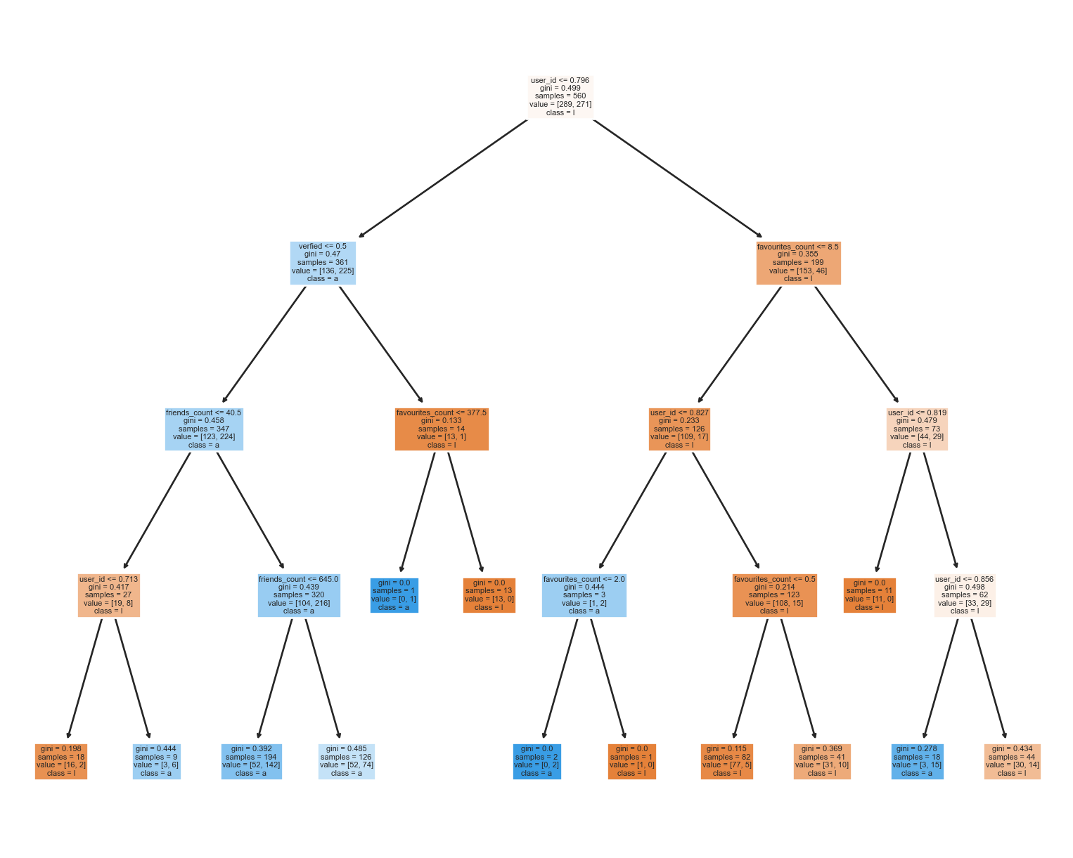
#fit the tree model with the best layer
model = tree.DecisionTreeClassifier(max_depth=4)
model = model.fit(x_train,y_train)

yp_train=model.predict(x_train)
yp_test=model.predict(x_test)

#write a function to visualize the confusion matrix
def confusion_plot(y_data,y_pred):
    print(
        "ACCURACY: "+str(accuracy_score(y_data,y_pred))+"\n"+
        "NEGATIVE RECALL (Y=0): "+str(recall_score(y_data,y_pred,pos_label=0))+"\n"+
        "NEGATIVE PRECISION (Y=0): "+str(precision_score(y_data,y_pred,pos_label=0))+"\n"+
        "POSITIVE RECALL (Y=1): "+str(recall_score(y_data,y_pred,pos_label=1))+"\n"+
        "POSITIVE PRECISION (Y=1): "+str(precision_score(y_data,y_pred,pos_label=1))+"\n"
    )
    cf=confusion_matrix(y_data, y_pred)
    # customize the anno
    group_names = ["True Neg","False Pos","False Neg","True Pos"]
    group_counts = ["{0:0.0f}".format(value) for value in cf.flatten()]
    group_percentages = ["{0:.2%}".format(value) for value in cf.flatten()/np.sum(cf)]
    labels = [f"{v1}\n{v2}\n{v3}" for v1, v2, v3 in zip(group_names,group_counts,group_percentages)]
    labels = np.asarray(labels).reshape(2,2)
    #plot the heatmap
    fig=sns.heatmap(cf, annot=labels, fmt="", cmap='Blues')
    plt.title("Confusion Matrix of Texts - Decision Tree",fontsize=18)
    fig.set_xticklabels(["Easily affected","Not easily affected"],fontsize=13)
    fig.set_yticklabels(["Easily affected","Not easily affected"],fontsize=13)
    fig.set_xlabel("Predicted Labels",fontsize=14)
    fig.set_ylabel("True Labels",fontsize=14)
    plt.show()
confusion_plot(y_test,yp_test)

#write a function to visualize the tree
def plot_tree(model,X,Y):
    fig = plt.figure(figsize=(10,8))
    tree_vis= tree.plot_tree(model, feature_names=X.columns,class_names=Y.name,filled=True)
plot_tree(model,x_test,y_test)

ACCURACY: 0.6357142857142857
NEGATIVE RECALL (Y=0): 0.4262295081967213
NEGATIVE PRECISION (Y=0): 0.6190476190476191
POSITIVE RECALL (Y=1): 0.7974683544303798
POSITIVE PRECISION (Y=1): 0.6428571428571429

With 4 layers, the leaf node seems quite reasonable.The model turns out to be quite trustable both on negative data. And favourite_count seems to be a remarkable metrics when grouping users.

Conclusion

The model is not bad. It can correctly distinguish most samples and the accuracy is about 70%. However, since our target is to find users easily be affected by rumors. A false positive is more acceptable than a false negative, which means it is more acceptable to warn a person not easily be affected than fail to notify a person who may trust a rumor and pass it along! So we can consider to apply this model.

Decision tree is unstable, so we can still use bagging(random forest), boosting(xgboost, GDBT, lightBGM, etc) to fit the data in the future.

Reference

[1]What is a decision tree. IBM. (n.d.). Retrieved December 4, 2022, from https://www.ibm.com/topics/decision-trees

Rumor & Susceptible User Detection

Introduction

Theory

Method

Class Distribution

Baseline Model for Comparsion

Data Selection

Model tuning

Final Results

Conclusion

Reference